MRI

This is an MRI scan of a human brain.

A sagittal MRI slice through a brain.

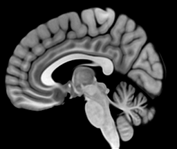
Drag through it and you can see the folds of the brain, the cerebellum tucked in at the back, and the brainstem running down toward the spine. How do you get a picture like this without opening the head?

The most common way to see inside a body is the X-ray. A beam of X-ray photons goes in one side of the body, and a plate on the other side records the ones that get through. The plate darkens wherever photons reach it, so anything that stops them leaves a pale shadow. Bone is full of calcium, and calcium atoms are heavy. A millimeter of bone stops about 4 times as many photons as a millimeter of brain, which puts bone close to rock.

A slice through a head seen from above, with a tumor in the brain, between an X-ray source on the left and an X-ray plate on the right.

So an X-ray gives you a picture of bone. But what if you want to see soft tissue, like the brain? Muscle, blood, brain, and tumors all stop photons within a few percent of each other. On the plate they make one flat gray, and a tumor in the brain leaves no trace.

You could try CT (computed tomography), which takes X-rays from many angles and computes a slice. Nothing in the slice overlaps, so it can show some soft tissue.² But it still measures how much each spot stops the beam, and soft tissues still differ by only a few percent.

If you’ve ever had an MRI, you might also wonder why it’s so different from getting an X-ray. An X-ray is over in a fraction of a second. For an MRI you lie in a narrow tube for 20 minutes or more, told not to move, while the machine knocks and buzzes around you. All of that comes from how the picture gets made.

The brain, the discs in the spine, and the ligaments in a knee are all mostly water. Maybe some property of water can tell them apart.

The scanner made the picture at the top out of the water in the head. Zoom in on one pixel and follow it down.

A sagittal MRI slice through a brain.

Each pixel stands for a voxel, a cube of brain less than a millimeter across. It holds tens of thousands of brain cells, and the cells are mostly water. Each water molecule has 2 hydrogen atoms. The nucleus of a hydrogen atom is a proton, and the protons are what the scanner listens to.

A proton is a tiny magnet. Its magnetic moment is the strength and direction of that magnet. A proton also spins about the same axis its magnet points along. Picture a spinning top that’s also a compass needle.

That matters because a moving magnet makes electricity. It’s how a generator works. Turn a magnet next to a coil of wire and a current flows back and forth in the wire. Stop the magnet and the current stops.

Interactive induction figure

Every turn makes a wave, and turning faster makes the waves taller. Every bit of data an MRI scan collects is a trace like this one.

So why not hold a coil up to someone’s head and listen to the protons directly? You’d hear nothing. Heat knocks the protons around constantly, so their magnets point every which way. For every proton pointing one way, there’s another pointing the opposite way, and they cancel. The water as a whole isn’t a magnet, and the coil has nothing to pick up.

For the coil to hear anything, the protons have to line up and turn together.

Magnets line up in a magnetic field, but heat keeps knocking the protons out of line. To beat the heat, the scanner needs a field tens of thousands of times stronger than Earth’s, 1.5 or 3 tesla. It makes one the way any electromagnet does, with current running around a coil of wire.

A coil of wire seen from above and cut through, with field lines running straight through the middle and spreading out past the ends, and a steel wrench resting off to one side.

The field is strong only inside the coil, so the scanner wraps a coil around you, and that’s the tube. Its field is called $B_0$ (“B naught”) and runs along the tube. The wire is superconducting, chilled in liquid helium so the current meets no resistance, and once started it flows for years. The magnet is always on, which is why steel never goes into the room. A wider tube would need a bigger coil and far more wire and helium, so it stays only a little wider than your shoulders.

Even 3 tesla barely wins. Only about 10 more protons per million point along the field than against it. That tiny surplus is the whole signal, and a stronger magnet lines up more protons.

The magnet lines up a few extra protons, and then they just sit there, pointing along $B_0$. A magnet that doesn’t move makes no current, so the coil still hears nothing. The scanner has to tip them over. Tilt a proton off the field and see what it does.

Interactive one-proton figure

The proton doesn’t fall back in line. It circles the field, and the circling is called precession. Tip all the lined-up protons over and they precess together, so the part of their magnet pointing sideways sweeps past the coil. The further they tip, the bigger that part. At 90° all of it points sideways, so that’s the tip the scanner wants.

The scanner can’t reach in and tilt them by hand. It can send in another magnetic field, though. Turning a magnet near a coil makes a current, and it works backward too. A current sent back and forth through a coil makes a magnetic field that flips back and forth with it. Flip it millions of times a second and it’s radio, and it passes right through the body.

This field is weak, about 100,000 times weaker than $B_0$, so one shove barely budges the protons. Small pushes can still add up if they come at the right times.

Interactive swing figure

In time, every push lands at the same point in the swing and adds to the last. At any other tempo, each push lands a little later than the one before, and soon they work against each other.

So what’s a proton’s rhythm? It’s the rate it precesses at, the Larmor frequency, $f_0$. It goes up in step with the field, the way turning up Field sped up the proton. For a proton it’s 42.58 MHz for every tesla, so at 3 tesla it’s about 128 million times a second.³ That’s a radio frequency, a little above the FM band.

The scanner’s radio coil is wired so its field turns in a circle instead of flipping back and forth. That field, $B_1$ (“B one”), lies sideways across $B_0$ and turns at the Larmor frequency. It keeps pace with the circling protons and pushes them from the same side every time around.

Interactive rf-pulse figure

The timing has to be close. A transmitter off by a few thousand turns a second, out of 128 million, barely moves the moment. It’s the swing pushed at the wrong tempo, so the pushes come from every side and cancel. That tight fit is the “resonance” in magnetic resonance imaging.

When the pulse stops, the moment spirals back toward $B_0$. A pulse can be over in under a millisecond, but the trip back takes anywhere from tens of milliseconds to a few seconds.

Now the coil can hear them. A precessing proton is the turning magnet from earlier, so it makes a current in a coil near the body. Tip it by different amounts and compare.

Interactive moment-signal figure

As the moment drifts back toward $B_0$, its sideways part shrinks and the wave fades with it.

One proton’s wave is far too small to pick out of the electrical noise in the coil. A coil hears nearby protons far better than distant ones, so the one that listens sits as close as it can. For a head scan, it’s the cage that fits over your face. It hears every proton near it at once. A droplet of water the size of a pinhead, 1 cubic millimeter, holds about 70 billion billion hydrogen atoms. Almost all of their moments cancel, but the few extra lined up along $B_0$ still number several hundred trillion.

What the coil hears is the total of all those moments. Arrows add tip to tail, and the total is the arrow from the first tail to the last tip. This total is the net magnetization, $M$.

Interactive sum-to-m figure

Opposite arrows cancel, and $M$ is what’s left, pointing along $B_0$. When the moments precess, $M$ stays put, so the coil hears nothing. A pulse tips every moment by the same angle, so $M$ tips over with them, and its sideways part sweeps past the coil.

Spin is really a quantum property, but $M$ averages over so many protons that the arrows describe it accurately. $M$ tips and circles like one arrow, but its length can change. If the moments point different ways, they add to a shorter total.

So the scanner can hear the water. But the coil hears every proton in the head mixed into one total, and nothing in that total says which protons it came from or where they are. A proton behind the eye and one at the back of the skull circle at the same rate, so they sound the same. To make a picture, the scanner has to make them sound different.

The scanner can change their rhythm, making protons in different places circle at slightly different rates. But next to 128 million turns a second, a difference of a few hundred is impossible to see. A camera that turns along with the protons takes away the shared motion and leaves only the differences. Someone riding a merry-go-round sees the horses stand still for the same reason.

Interactive rotating-frame figure

The room’s view is called the lab frame, and the turning camera’s view is the rotating frame. In the rotating frame, $B_1$ stands still too, since it turns at the same rate, and the pulse tips the moment slowly over around it. The coil doesn’t turn with the camera, so switching cameras changes nothing about the signal, only how easy it is to see.

How does the scanner pick out one part of the head? It already has a way to pick. A pulse only tips protons whose rhythm matches the transmitter, and their rhythm goes up with the field. The transmitter here stays at 64 MHz. Slide Field $B_0$ and see where the pulse starts to work.

Interactive rf-field figure

The pulse only tips the moment near 1.5 tesla, where the field brings it into tune. So the scanner makes the field a little stronger on one side of the head than the other, using a second set of coils inside the magnet, the gradient coils. That change in strength from place to place is called a gradient. Now a pulse tips one slab of the head, a few millimeters thick, and leaves the rest alone. A new transmitter frequency moves the slab, and a stronger gradient makes it thinner. This is slice selection, and it’s how the side-view slice near the top of the article was picked.

That leaves the spots inside the slice, which still add into one total. To tell them apart, the scanner turns a gradient on again after the pulse, while the protons are circling. Take 3 small samples of water at different spots along it.

Three fixed samples with vertical magnetic field arrows and transverse magnetization arrows. A gradient changes their relative precession rates.

With the gradient on, each sample precesses at its own rate, depending on where it sits. Turn the gradient off and the rates match again, but the samples keep the angles they’ve picked up. Turn it on in the opposite direction and those angles unwind. The scanner controls how strong each gradient is and how long it stays on.

In a real scanner, every one of those switches is loud. The gradient coils carry hundreds of amps and switch in under a millisecond. The wire sits in the main field, so each switch shoves it sideways, and the knocking you hear in a scanner is the coils flexing with each shove.

Each sample’s angle now depends on where it sits, but the coil still hears only their total.

Line up a row of samples across the slice and look down on them from above. Each $M$ is now a hand on a dial. The large hand, total $M$, is their sum, the only thing the coil hears. Switch the gradient on and watch what the total does.

A row of 20 samples seen from above, each with a clock hand, winding into a stripe pattern under a gradient. Below them one large hand shows their total, and a trace records its length.

The gradient winds the row up. After 1 full turn, the hands go once around the dial from one end of the row to the other, and after 2 turns they go around twice. Each whole number of turns lays a stripe pattern over the row, with that many stripes. How far the row winds depends on the gradient’s strength times how long it’s on, called the gradient area.

At every whole turn the total drops to zero, even though every hand is still tipped and full length. They point every way around the dial and cancel. Reverse the gradient and the row unwinds, and the total comes back.

Real tissue doesn’t hold the same water everywhere. Where there’s more water the hands are longer, so at a whole turn they don’t cancel. What’s left says how much the water matches that stripe pattern.

Any picture can be built from stripe patterns, starting with a flat level, then 1 stripe across, then 2, and so on, each with its own strength and position. So a scanner that measures every stripe pattern in the water can add them back up into the picture.

A row of 31 dials shaded by their water, each with a clock hand, over a strip of gray cells, a curve of the sum so far over the water, and a large dial showing their total. Beneath, a stack of patterns fills in as the twist passes whole turns.

At zero twist all the hands agree, and the total is the average water, the flat level. This row also has a ripple of 6 bumps. At 6 turns, the hands on the bumps point one way and the hands between them point the other. The bumps hold more water, so the two sides don’t cancel. The total’s length says how big the ripple is, and its angle says where the bumps sit.

The first few turns give the rough shape, and later turns sharpen the edges. Finer detail needs more turns, and more turns need more gradient area, so sharper images take longer to read out.

A slice isn’t one row, though. It has rows stacked down it too. The scanner covers that direction with a second gradient, which winds the hands from top to bottom. With a twist across and a twist down at the same time, the stripes run at an angle. Every pair of twists is its own stripe pattern, and together they make a map.

So how does the scanner get around the map? The current pair of twists is a marker on it. The 2 gradients move the marker while they’re on, and it stays put while they’re off. The coil is read at a steady rate wherever the marker is. Try steering it yourself.

Three panels: the sagittal slice at 31 pixels across, an empty picture, and an empty map, with a round pad and knob below. Dots land on the map and the picture fills in as the marker moves.

The middle of the map gives the biggest readings, because at small twists the hands still mostly agree. Readings at the edge are about 10,000 times smaller. A path through the middle already gives the shape of the head, and a path along the edge gives only fine detail. The marker also has a top speed, because the gradients can only get so strong. Drag faster than that and the marker falls behind.

Press play to see the scanner’s own path. After each pulse, 2 short gradients carry the marker to the left end of a row, and a steady gradient sweeps it across while the coil records. The biggest dot in each row is where the sweep unwinds the twist across and the total comes back, called an echo. Rows go top to bottom, so the picture is only stripes until the middle rows land.

The slice at the top of the article is 256 by 256 pixels, so its map has 256 by 256 points. Each point is a stripe pattern over the whole head, and its weight is the total the scanner measured there.

Three panels: the sagittal slice being built from its patterns, the stripe pattern at a chosen point of the map, and the map itself on a log scale with a marker.

Keep only the rim of the map and the image is an outline.

In symbols, let $w_k$ and ${\theta }_k$ be the length and angle of the weight of pattern $k$, and let $k_x$ and $k_y$ be its twists. Then

$$\text{image}(x,y)=\sum _k{w}_k\cos (2\pi (k_{x}x+k_{y}y)+{\theta }_k)$$

This sum is a Fourier transform, and the map is called k-space. Doing the sum directly for this slice takes about 4 billion multiplications. The fast Fourier transform does it in a few million, so the image is ready seconds after the scan.

Every one of the 65,536 pixels is built from all 65,536 readings, because each pattern covers the whole slice. That’s why you have to hold still. If your head moves during row 200, the readings after that describe a head in a slightly different place. Adding them to the first 199 smears the mismatch across the whole image, not just the part that moved.

So why does it take so long? A 256-row map needs 256 pulses. Before each one, the scanner waits for the protons to spiral back toward $B_0$, the trip that takes up to a few seconds. At about a second a row, that’s 4 minutes for 1 slice. Scanners fill other slices during the wait, so a whole stack takes about as long, and an exam is several of these scans back to back.

The wait also changes what the image shows, because tissues recover and lose signal at different rates. When the scanner pulses and when it listens decides which tissues are bright. This is contrast, and the next article starts there.